Efficient vector similarity search with Redis: a step-by-step tutorial

Wednesday, February 22, 2023 by ezzcodeezzlife

Enhancing search results with vector embeddings and Redis

The ability to search for information is crucial in today's digital landscape, with users expecting search functionality in nearly every application and website. To improve search results, architects and developers must continuously explore new methods and architectures. One of the approaches is to utilize vector embeddings generated by deep learning models, which can enhance the accuracy and relevance of search results.

To this end, many organizations are leveraging indexing techniques to transform their data into vector space. By representing data as vectors, it becomes possible to perform similarity searches that return the most relevant results.

In this tutorial, we will explore how deep learning models can be used to create vector embeddings, which can then be indexed for efficient and accurate search with the help of Redis. With a thorough understanding of this approach, architects and developers can better appreciate the potential of AI-powered search capabilities and find best ways to improve the search experience for users.

We will go through the process of:

creating vector embeddings for Amazon product dataset,
indexing them with Redis
searching for similar vectors.

We will also explore the pros and cons of different indexing methods and how they can be used to improve search performance.

Let's get started!

Create a new directory and create a new Jupyter notebook. Get the dataset CSV file from here. Store it in ./data/ dir. We will be using Python 3.8. Install the following dependencies in the first cell:

%pip install redis numpy pandas
%pip install -U sentence-transformers

After installing the dependencies, you can start by importing the necessary libraries and defining any necessary classes or functions. In this case, we can import the following libraries and define a color class for later use:

import random
import numpy as np
import pandas as pd
import time
from redis import Redis
from redis.commands.search.field import VectorField
from redis.commands.search.field import TextField
from redis.commands.search.field import TagField
from redis.commands.search.query import Query
from redis.commands.search.result import Result

class color:
   PURPLE = '\033[95m'
   CYAN = '\033[96m'
   DARKCYAN = '\033[36m'
   BLUE = '\033[94m'
   GREEN = '\033[92m'
   YELLOW = '\033[93m'
   RED = '\033[91m'
   BOLD = '\033[1m'
   UNDERLINE = '\033[4m'
   END = '\033[0m'

The Redis library is imported to interact with Redis, an in-memory data structure store often used as a database, cache, and message broker. We also import the following classes from redis.commands.search.field and redis.commands.search.query modules:

VectorField: used to represent vector fields in Redis, such as embeddings.
TextField: used to represent text fields in Redis.
TagField: used to represent tag fields in Redis.
Query: used to create search queries for Redis.
Result: used to represent search results returned by Redis.

In addition, we define a color class that can be used to print colored text to the console. The color class has several attributes, such as PURPLE, CYAN, BOLD, etc., which can be used to colorize text output in the console.

The next step involves loading Amazon product data into a Pandas DataFrame, and truncating long text fields to a maximum length of 512 characters, which is the maximum length supported by the pre-trained sentence embedding generator that we will be using later on.

Here's the cell code to load the product data and truncate long text fields:

MAX_TEXT_LENGTH = 512
NUMBER_PRODUCTS = 1000

# define a function to auto-truncate long text fields
def auto_truncate(val):
    return val[:MAX_TEXT_LENGTH]

# load the product data and truncate long text fields
all_prods_df = pd.read_csv("data/product_data.csv", converters={'bullet_point': auto_truncate, 'item_keywords': auto_truncate, 'item_name': auto_truncate})
all_prods_df['primary_key'] = all_prods_df['item_id'] + '-' + all_prods_df['domain_name']
all_prods_df['item_keywords'].replace('', np.nan, inplace=True)
all_prods_df.dropna(subset=['item_keywords'], inplace=True)
all_prods_df.reset_index(drop=True, inplace=True)

# get the first 1000 products with non-empty item keywords
product_metadata = all_prods_df.head(NUMBER_PRODUCTS).to_dict(orient='index')

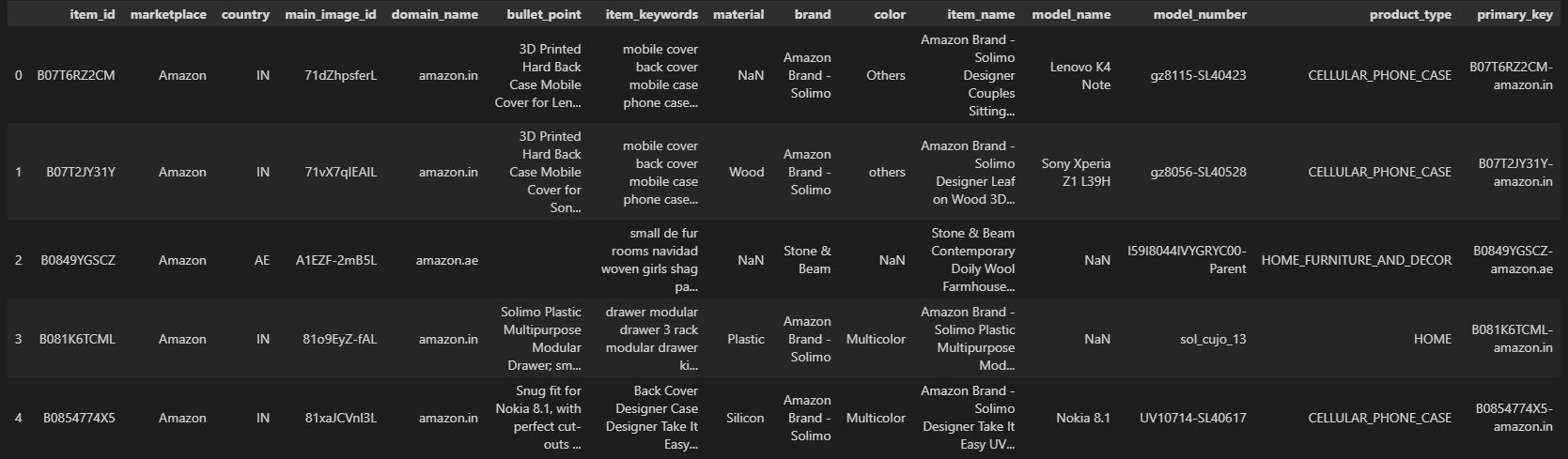
The code loads the product data from a CSV file, truncates long text fields, adds a new primary_key column to the DataFrame, filters out any products without keywords, and extracts the metadata for the first 1000 products with non-empty item keywords and stores it in a dictionary called product_metadata.

Let's take a look at the first few rows of the product data:

all_prods_df.head()

Connect to Redis

After loading the product data into a Pandas DataFrame and extracting metadata for the 1000 products, the next step is to connect to Redis. We will be using a Redis instance provided by RedisLabs in their cloud, which offers a free tier. You can sign up for a free account at redis.com/try-free/.

Spin up a new Redis instance and copy the connection details. You will need to provide a password when connecting to the Redis instance. You can find the password in the connection details page. The password is the same as the password for the default user.

redis_conn = Redis(
  host='XXX',
  port=XXXXX,
  password="<YOUR-DEFAULT-USER-PW>")
print ('Connected to redis')

Create embeddings

Using SentenceTransformer

The next step involves generating embeddings (vectors) for the item keywords using a pre-trained Sentence Transformer model called distilroberta-v1. This model is available from the Sentence Transformer library. We will use the SentenceTransformer class to load the model and generate the embeddings.

from sentence_transformers import SentenceTransformer
model = SentenceTransformer('sentence-transformers/all-distilroberta-v1')

%%time

item_keywords =  [product_metadata[i]['item_keywords']  for i in product_metadata.keys()]
item_keywords_vectors = [ model.encode(sentence) for sentence in item_keywords]

Then we will check the dimensions of the embeddings:

len(item_keywords_vectors)
len(product_metadata)
# Check one of the products
product_metadata[0]

Preparing utility functions

Now we have 1000 embeddings for the 1000 products. Next, we will define 3 utility functions. One for loading the product data and two for creating the index on Vector fields.

def load_vectors(client:Redis, product_metadata, vector_dict, vector_field_name):
    p = client.pipeline(transaction=False)
    for index in product_metadata.keys():    
        #hash key
        key='product:'+ str(index)+ ':' + product_metadata[index]['primary_key']
        
        #hash values
        item_metadata = product_metadata[index]
        item_keywords_vector = vector_dict[index].astype(np.float32).tobytes()
        item_metadata[vector_field_name]=item_keywords_vector
        
        # HSET
        p.hset(key,mapping=item_metadata)
            
    p.execute()

def create_flat_index (redis_conn,vector_field_name,number_of_vectors, vector_dimensions=512, distance_metric='L2'):
    redis_conn.ft().create_index([
        VectorField(vector_field_name, "FLAT", {"TYPE": "FLOAT32", "DIM": vector_dimensions, "DISTANCE_METRIC": distance_metric, "INITIAL_CAP": number_of_vectors, "BLOCK_SIZE":number_of_vectors }),
        TagField("product_type"),
        TextField("item_name"),
        TextField("item_keywords"),
        TagField("country")        
    ])

def create_hnsw_index (redis_conn,vector_field_name,number_of_vectors, vector_dimensions=512, distance_metric='L2',M=40,EF=200):
    redis_conn.ft().create_index([
        VectorField(vector_field_name, "HNSW", {"TYPE": "FLOAT32", "DIM": vector_dimensions, "DISTANCE_METRIC": distance_metric, "INITIAL_CAP": number_of_vectors, "M": M, "EF_CONSTRUCTION": EF}),
        TagField("product_type"),
        TextField("item_keywords"),        
        TextField("item_name"),
        TagField("country")     
    ])

Comparison of flat and HNSW indexing for approximate nearest neighbor search

Flat indexing and HNSW are both methods used in approximate nearest neighbor search in high-dimensional spaces, but they differ in the way they construct and search the index.

Flat indexing is a straightforward approach where all data points are indexed and stored in a single list or tree structure. To find the nearest neighbors of a query point, a brute force search is conducted by computing the distance between the query point and all other points in the index. While simple and easy to implement, flat indexing can be computationally expensive and impractical for large datasets and high-dimensional spaces.

HNSW, on the other hand, stands for Hierarchical Navigable Small World and is a more complex indexing algorithm that organizes data points into a hierarchical graph structure. This graph is built by connecting each point to its nearest neighbors, and then recursively connecting nearby points in a hierarchical manner. This results in a graph structure that is highly clustered and enables fast approximate nearest neighbor search by exploring only a small subset of the graph.

The key advantage of HNSW over flat indexing is its ability to scale to large datasets and high-dimensional spaces. However, HNSW requires more careful tuning of its parameters and may have higher index construction time compared to flat indexing.

Index & Query the new data

Next, we will load and index the product data using a flat index first.

%%time

ITEM_KEYWORD_EMBEDDING_FIELD='item_keyword_vector'
TEXT_EMBEDDING_DIMENSION=768
NUMBER_PRODUCTS=1000

print ('Loading and Indexing + ' +  str(NUMBER_PRODUCTS) + ' products')

#flush all data
redis_conn.flushall()

#create flat index & load vectors
create_flat_index(redis_conn, ITEM_KEYWORD_EMBEDDING_FIELD,NUMBER_PRODUCTS,TEXT_EMBEDDING_DIMENSION,'COSINE')
load_vectors(redis_conn,product_metadata,item_keywords_vectors,ITEM_KEYWORD_EMBEDDING_FIELD)

Query our FLAT index

And after this we can query our index and search for the top 5 (topK) nearest neighbors for a given query vector:

%%time
topK=5
product_query='beautifully crafted present for her. a special occasion'
#product_query='cool way to pimp up my cell'

#vectorize the query
query_vector = model.encode(product_query).astype(np.float32).tobytes()

#prepare the query
q = Query(f'*=>[KNN {topK} @{ITEM_KEYWORD_EMBEDDING_FIELD} $vec_param AS vector_score]').sort_by('vector_score').paging(0,topK).return_fields('vector_score','item_name','item_id','item_keywords').dialect(2)
params_dict = {"vec_param": query_vector}


#Execute the query
results = redis_conn.ft().search(q, query_params = params_dict)

#Print similar products found
for product in results.docs:
    print ('***************Product  found ************')
    print (color.BOLD + 'hash key = ' +  color.END + product.id)
    print (color.YELLOW + 'Item Name = ' +  color.END  + product.item_name)
    print (color.YELLOW + 'Item Id = ' +  color.END  + product.item_id)
    print (color.YELLOW + 'Item keywords = ' +  color.END  + product.item_keywords)
    print (color.YELLOW + 'Score = ' +  color.END  + product.vector_score)

***************Product  found ************
hash key = product:597:B076ZYG35R-amazon.com
Item Name = Amazon Brand - The Fix Women&#39;s Lizzie Block Heel Ruffled Sandal Heeled, Dove Suede, 9 B US
Item Id = B076ZYG35R
Item keywords = gifts her zapatos shoe ladies mujer womans designer spring summer date night dressy fancy high heels
Score = 0.498145997524

***************Product  found ************
hash key = product:112:B07716JGFN-amazon.com
Item Name = Amazon Brand - The Fix Women&#39;s Jackelyn Kitten Heel Bow Sandal Heeled
Item Id = B07716JGFN
Item keywords = zapatos shoe ladies mujer womans spring summer casual date night gifts for her
Score = 0.613550662994

***************Product  found ************
hash key = product:838:B0746M8ZY9-amazon.com
Item Name = Amazon Brand - 206 Collective Women&#39;s Roosevelt Shearling Slide Slipper Shoe, Chestnut, 7.5 B US
Item Id = B0746M8ZY9
Item keywords = zapatos shoe para de ladies mujer womans mocasines designer  clothing  work wear office top gifts gifts for gifts for her
Score = 0.623450696468

***************Product  found ************
hash key = product:800:B0065HI4KA-amazon.com
Item Name = Sterling Silver Ribbon Black and White Diamond Earrings (1/5 cttw, I-J Color, I2-I3 Clarity)
Item Id = B0065HI4KA
Item keywords = classics with a twist braid twist rope color diamonds black diamonds valentines day gifts for her valentines day jewelry valentines day love gifts for women valentine jewelry valentines jewelry gifts for her braided earrings rope earrings black diamond earrings color diamond earrings braid twist rope color diamonds black diamonds valentines day gifts for her valentines day jewelry valentines day love gifts for women valentine jewelry valentines jewelry gifts for her braided earrings rope earrings black diam
Score = 0.628378272057

***************Product  found ************
hash key = product:475:B07DJ2M9YR-amazon.com
Item Name = Essentials Women&#39;s Pom Knit Hat and Scarf Set
Item Id = 0mB07DJ2M9YR
Item keywords = women woman ladies winter gift cozy
Score = 0.644373476505

Query our HNSW index

It's working! That's great! Now let's try the same with HNSW indexing. First Load and index product data.

%%time
print ('Loading and Indexing + ' +  str(NUMBER_PRODUCTS) + ' products')

ITEM_KEYWORD_EMBEDDING_FIELD='item_keyword_vector'
NUMBER_PRODUCTS=1000
TEXT_EMBEDDING_DIMENSION=768

#flush all data
redis_conn.flushall()

#create flat index & load vectors
create_hnsw_index(redis_conn, ITEM_KEYWORD_EMBEDDING_FIELD,NUMBER_PRODUCTS,TEXT_EMBEDDING_DIMENSION,'COSINE',M=40,EF=200)
load_vectors(redis_conn,product_metadata,item_keywords_vectors,ITEM_KEYWORD_EMBEDDING_FIELD)

And now we can query again:

%%time
topK=5
product_query='beautifully crafted present for her. a special occasion'
#product_query='cool way to pimp up my cell'

#vectorize the query
query_vector = model.encode(product_query).astype(np.float32).tobytes()

#prepare the query
q = Query(f'*=>[KNN {topK} @{ITEM_KEYWORD_EMBEDDING_FIELD} $vec_param AS vector_score]').sort_by('vector_score').paging(0,topK).return_fields('vector_score','item_name','item_id','item_keywords','country').dialect(2)
params_dict = {"vec_param": query_vector}


#Execute the query
results = redis_conn.ft().search(q, query_params = params_dict)

#Print similar products found
for product in results.docs:
    print ('***************Product  found ************')
    print (color.BOLD + 'hash key = ' +  color.END + product.id)
    print (color.YELLOW + 'Item Name = ' +  color.END  + product.item_name)
    print (color.YELLOW + 'Item Id = ' +  color.END  + product.item_id)
    print (color.YELLOW + 'Item keywords = ' +  color.END  + product.item_keywords)
    print (color.YELLOW + 'Country = ' +  color.END  + product.country)
    print (color.YELLOW + 'Score = ' +  color.END  + product.vector_score)

Learn more!

You can find the full code in this Github repository. We highly recommend checking out
this repo for more information and a guide on how to do a similarity search like we did here with images.

Thank you! If you enjoyed this tutorial you can find more and continue reading on our tutorial page. And if you want to check what you have learnt right away I strongly recommend joining one of our AI hackathons. - Fabian Stehle, Developer at New Native