Fine-Tuning TinyLLaMA with Unsloth
Fine-Tuning TinyLLaMA with Unsloth: A Hands-On Guide
Hey there, folks! 👋 Tommy here, ready to dive into the exciting world of fine-tuning TinyLLaMA, a Small Language Model (SLM) optimized for edge devices like mobile phones. Whether you’re an intermediate developer, AI enthusiast, or gearing up for your next hackathon project, this tutorial will walk you through everything you need to know to fine-tune TinyLLaMA using Unsloth.
Now Let's get started! 🚀
Prerequisites 🧠
Before we jump into the tutorial, make sure you have the following:
- Basic Python Knowledge
- Familiarity with Machine Learning Concepts
- A Google account for accessing Google Colab.
- A W&B account (you can sign up here).
Setting Up Fine-Tuning Environment 🛠️
We’ll use Google Colab to fine-tune TinyLLaMA, which offers a free and accessible GPU for this process. Here’s how to get started:
Create a New Colab Notebook:
First, head over to Google Colab and create a new notebook.
Next, ensure you have a GPU available by setting the notebook's runtime to use a GPU. You can do this by going to the menu and selecting Runtime > Change runtime type. In the window that appears, choose T4 GPU from the Hardware accelerator section.
Install Dependencies:
Now we need to install the required libraries and dependencies. Run the command below in your code cell:
 !pip install "unsloth[colab-new] @ git+https://github.com/unslothai/unsloth.git"
 !pip install --no-deps "xformers<0.0.27" "trl<0.9.0" peft accelerate bitsandbytes
Loading the Model and Tokenizer 🧩
After setting up your environment, the next step is to load the TinyLLaMA model and its tokenizer.
Here’s how to load the TinyLLaMA model with some configuration options:
from unsloth import FastLanguageModel
import torch

# Configuration settings
max_seq_length = 2048  # Maximum sequence length supported by the model
dtype = None           # Set to None for auto-detection, Float16 for T4/V100, Bfloat16 for Ampere GPUs
load_in_4bit = True    # Enable 4-bit loading for memory efficiency

# Load the model and tokenizer
model, tokenizer = FastLanguageModel.from_pretrained(
    model_name="unsloth/tinyllama-bnb-4bit",  # Model name for 4-bit precision loading
    max_seq_length=max_seq_length,
    dtype=dtype,
    load_in_4bit=load_in_4bit,
    # token = "hf_...", # Uncomment and use if working with gated models like Meta's LLaMA-2
)
Layer Selection and Hyperparameters ⚙️
After loading the model, the next step involves configuring it for fine-tuning by selecting specific layers and setting key hyperparameters. We'll be using the get_peft_model method from the FastLanguageModel provided by Unsloth. This method allows us to apply Parameter-Efficient Fine-Tuning (PEFT) techniques, specifically Low-Rank Adaptation (LoRA), which helps in adapting the model with fewer parameters while maintaining performance.
Here's the code to configure the model:
model = FastLanguageModel.get_peft_model(
    model,
    r=16,  # LoRA rank, affects the number of trainable parameters
    target_modules=["q_proj", "k_proj", "v_proj", "o_proj",
                    "gate_proj", "up_proj", "down_proj"],
    lora_alpha=16,
    lora_dropout=0,  # Dropout for regularization, currently set to 0
    bias="none",     # No bias used in this configuration
    use_gradient_checkpointing=True,  # Useful for reducing memory usage during training
    use_rslora=False,  # Rank Stabilized LoRA, set to False in this case
    loftq_config=None, # LoRA with Quantization, not used here
)
When fine-tuning TinyLLaMA, special attention should be given to the attention and feed-forward layers:
- Attention Layers: These layers are key to how TinyLLaMA focuses on different parts of the input. By fine-tuning these layers, you help the model better understand and contextualize the data. Example of the layers used are "q_proj", "k_proj", "v_proj", "o_proj"
- Feed-Forward Layers: These layers handle the transformations post-attention, crucial for the model’s ability to process and generate complex outputs. Optimizing these layers can greatly enhance performance on specific tasks. Examples of the layers used are: "gate_proj", "up_proj", "down_proj"
Preparing the Dataset and Defining the Prompt Format 📝
After configuring your model, the next step is to prepare your dataset and define the prompt format. For this tutorial, we'll use the Alpaca dataset from Hugging Face, but I'll also show you how to create and load a custom dataset if you want to use your own data.
Using the Alpaca Dataset
The Alpaca dataset is designed for training models to follow instructions. We’ll load it directly from Hugging Face and format it according to the structure expected by the TinyLLaMA model.
Here's the code to load and format the Alpaca dataset:
from datasets import load_dataset

# Load the Alpaca dataset from Hugging Face
dataset = load_dataset("tatsu-lab/alpaca", split="train")

# Define a prompt template
alpaca_prompt = """Below is an instruction that describes a task, paired with an input that provides further context. Write a response that appropriately completes the request.

### Instruction:
{}

### Input:
{}

### Response:
{}"""

EOS_TOKEN = tokenizer.eos_token

# Function to format the prompts
def formatting_prompts_func(examples):
    instructions = examples["instruction"]
    inputs       = examples["input"]
    outputs      = examples["output"]
    texts = []
    for instruction, input, output in zip(instructions, inputs, outputs):
        # Must add EOS_TOKEN, otherwise your generation will go on forever!
        text = alpaca_prompt.format(instruction, input, output) + EOS_TOKEN
        texts.append(text)
    return { "text" : texts, }

# Apply the formatting function to the dataset
dataset = dataset.map(formatting_prompts_func, batched=True)

# Split the dataset into training and testing sets
dataset_dict = dataset.train_test_split(test_size=0.005)

train_dataset = dataset_dict[“train”]
eval_dataset = dataset_dict[“test”]
Creating and Loading a Custom Dataset
If you want to use your own custom dataset, you can easily do so by following these steps:
- Create a JSON file with your data. The file should contain a list of objects, each with
instruction,input, andoutputfields. For example:
[
    {
        "instruction": "Translate the following English text to French.",
        "input": "Hello, how are you?",
        "output": "Bonjour, comment ça va?"
    },
    {
        "instruction": "Summarize the following article.",
        "input": "In a recent study, scientists discovered...",
        "output": "Scientists discovered new findings in a recent study..."
    }
]
- Save this JSON file, for example as
dataset.json. - Load the custom dataset using the
load_datasetfunction from the Hugging Facedatasetslibrary:
from datasets import load_dataset

# Load your custom dataset from a JSON file
dataset = load_dataset("json", data_files="path/to/dataset.json")
Monitoring Fine-Tuning with W&B 📊
Weights & Biases (W&B) is an essential tool for tracking your model's training process and system resource usage. It helps visualize metrics in real time, providing valuable insights into both model performance and GPU utilization.
We'll use W&B to monitor our training process, including evaluation metrics and resource usage:
import wandb

# Log in to W&B - you'll be prompted to input your API key
wandb.login()

# Set W&B environment variables
%env WANDB_WATCH=all
%env WANDB_SILENT=true
You can sign up for W&B and get your API key here. This setup will allow you to track all the important metrics in real-time.
Training TinyLLaMA with W&B Integration
Now that everything is set up, it’s time to train the TinyLLaMA model. We'll be using the SFTTrainer from the trl library, along with Weights & Biases (W&B) for real-time tracking of training metrics and resource usage. This step ensures you can monitor your training effectively and make necessary adjustments on the fly.
Initializing W&B and Setting Training Arguments
First, we initialize W&B and set up the training arguments:
from trl import SFTTrainer
from transformers import TrainingArguments
from unsloth import is_bfloat16_supported
from transformers.utils import logging
import wandb

logging.set_verbosity_info()

# Initialize W&B
project_name = "tiny-llama"
entity = "wandb"
wandb.init(project=project_name, name="unsloth-tiny-llama")

# Define training arguments
training_args = TrainingArguments(
    per_device_train_batch_size=2,           # Small batch size due to limited GPU memory
    gradient_accumulation_steps=4,           # Accumulate gradients over 4 steps
    evaluation_strategy="steps",             # Evaluate after a certain number of steps
    warmup_ratio=0.1,                        # Warm-up learning rate over 10% of training
    num_train_epochs=1,                      # Number of epochs
    learning_rate=2e-4,                      # Learning rate for the optimizer
    fp16=not is_bfloat16_supported(),        # Use FP16 if BF16 is not supported
    bf16=is_bfloat16_supported(),            # Use BF16 if supported (more efficient on Ampere GPUs)
    max_steps=20,                            # Cap training at 20 steps for quick experimentation, increase or comment out as you see fit
    logging_steps=1,                         # Log metrics every step
    optim="adamw_8bit",                      # Use 8-bit AdamW optimizer to save memory
    weight_decay=0.1,                        # Regularization to avoid overfitting
    lr_scheduler_type="linear",              # Use linear learning rate decay
    seed=3407,                               # Random seed for reproducibility
    report_to="wandb",                       # Enable logging to W&B
    output_dir="outputs",                    # Directory to save model outputs
)
Next, we set up the SFTTrainer:
trainer = SFTTrainer(
    model=model,
    tokenizer=tokenizer,
    train_dataset=train_dataset,     # Training dataset
    eval_dataset=eval_dataset,       # Evaluation dataset
    dataset_text_field="text",               # The field containing text in the dataset
    max_seq_length=max_seq_length,           # Max sequence length for inputs
    dataset_num_proc=2,                      # Number of processes for dataset loading
    packing=True,                            # Packs short sequences together to save time
    args=training_args,                      # Training arguments defined earlier
)
Here’s how to efficiently manage the training process:
- Batch Size and Gradient Accumulation: Due to the limited memory of the GPU (especially in a free Colab environment), keep the batch size small. Use gradient accumulation to simulate a larger batch size, which stabilizes training without running out of memory.
- Mixed Precision Training: Utilize mixed precision (FP16 or BF16) to reduce memory usage and speed up training, particularly on modern GPUs like Tesla T4 or Ampere-based GPUs.
- Efficient Resource Management: By using 4-bit quantization (
load_in_4bit=True) and 8-bit optimizers, you significantly reduce the memory footprint, allowing for more efficient training on smaller devices. - Logging and Monitoring: W&B provides real-time monitoring of training metrics such as loss, accuracy, and resource usage (CPU/GPU). Use this to keep an eye on the training dynamics and adjust hyperparameters if needed.
- Evaluation Strategy: Set the evaluation strategy to
"steps"so that the model is evaluated periodically during training, allowing you to monitor its progress and prevent overfitting early on.
Once everything is set up, start the training loop. Once the training is complete, you can use the model as needed, and don't forget to properly close out your Weights & Biases (W&B) session.
# Start training the model
trainer.train()

# Finish and close the W&B session
wandb.finish()
Monitoring Training with Weights & Biases (W&B)
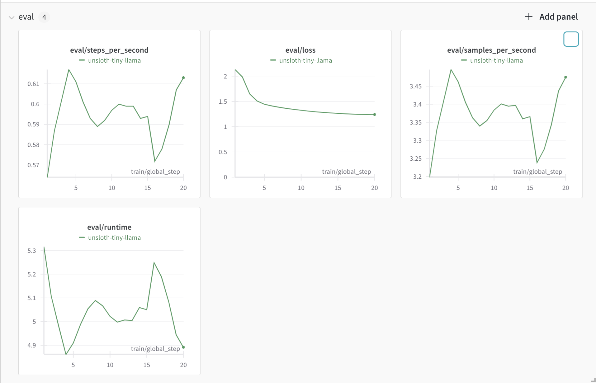
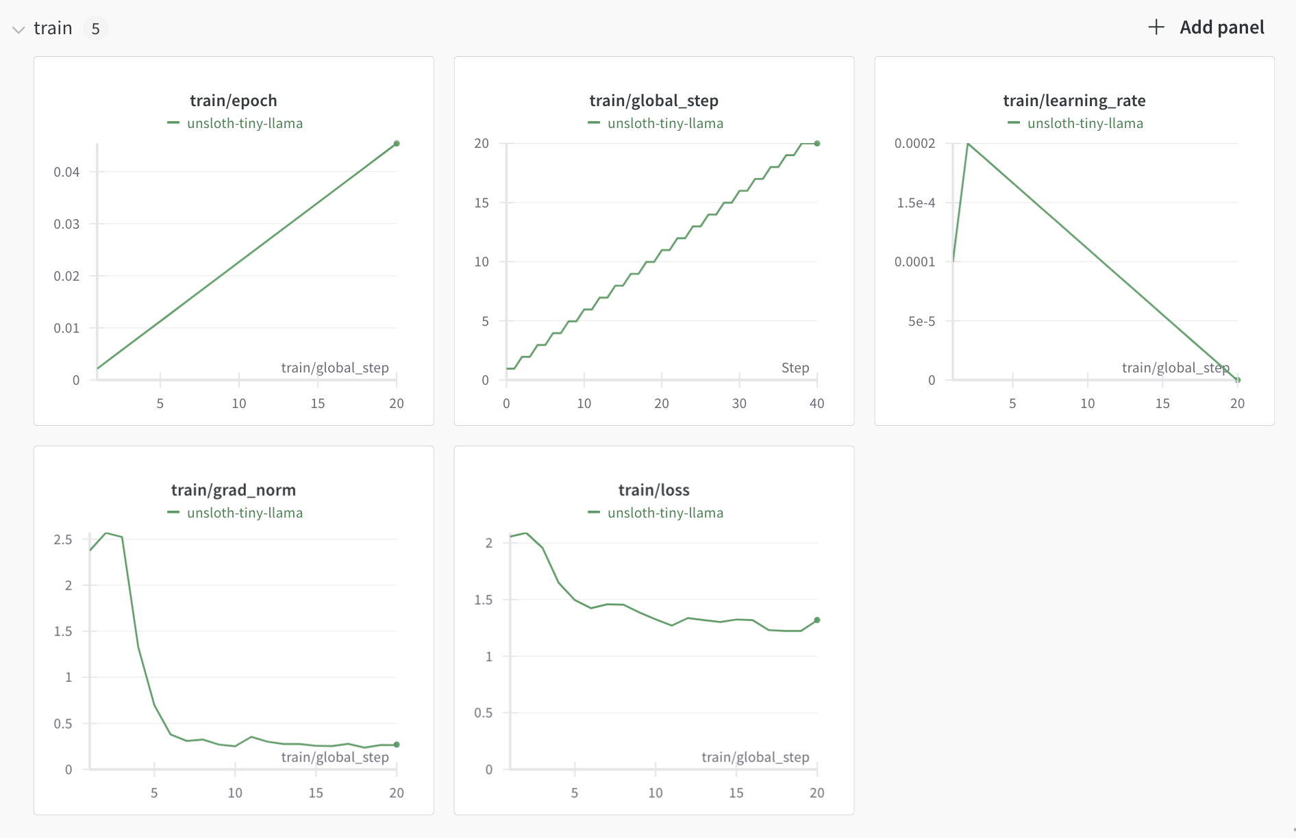
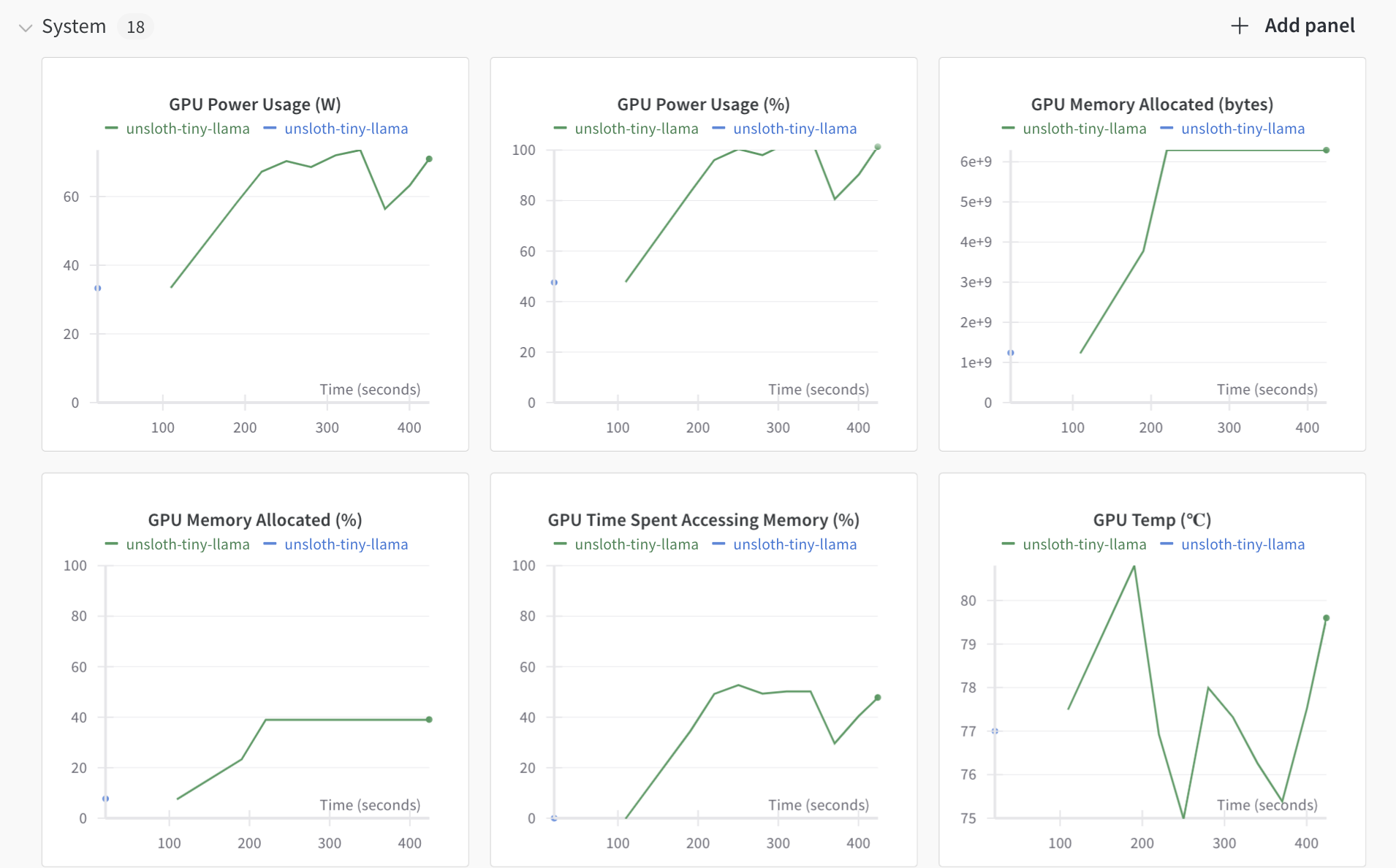
After integrating W&B into your training script, you can easily monitor various metrics from the W&B dashboard.
To view and interpret these metrics:
- Log in to W&B: Once your training starts, log in to the W&B website.
- Navigate to Your Project: In your workspace, locate the project you've set up (e.g., "tiny-llama") and click on it.
- Explore the Dashboard: In the
eval,train, andsystemsections, you’ll find a variety of metrics visualized over time.
Interpretation of Metrics
Evaluation Metrics:
- Loss: Monitoring this helps identify overfitting—if this loss starts increasing while training loss decreases, it suggests overfitting.
- Steps per Second: Measures training speed, helping optimize computational efficiency.

Training Metrics:
- Loss: Indicates how well the model learns from the training data. A decreasing loss typically indicates that the model is learning, but a very low loss might suggest overfitting.
- Learning Rate: Adjusts during training to ensure model convergence without overshooting.

System Resource Usage:
- GPU Power and Memory Usage: Visualize how your model utilizes the GPU. High and stable usage suggests efficient training.

Testing the Fine Tuned Model
After fine-tuning your model, you can test its performance with the following code:
FastLanguageModel.for_inference(model)  # Enable faster inference
inputs = tokenizer(
    [
        alpaca_prompt.format(
            "What is the capital of Spain?",  # instruction
            "",  # input
            "",  # output - leave this blank for generation!
        )
    ], return_tensors="pt"
).to("cuda")

outputs = model.generate(**inputs, max_new_tokens=64, use_cache=True)
outputs = tokenizer.decode(outputs[0])
print(outputs)
Before and After Fine-Tuning
- Before Fine-Tuning: The model doesn’t give any response at all.

- After Fine-Tuning: The model should provide accurate and contextually appropriate answers.

Saving the Fine-Tuned Model
The next step is to save the model. You can save the model locally or push it to the Hugging Face Hub for easy sharing and future use. Here’s how you can do both:
Saving the Model Locally
To save the model and tokenizer locally:
model.save_pretrained("path/to/save/directory")
tokenizer.save_pretrained("path/to/save/directory")
This will store your fine-tuned model and tokenizer in the specified directory. You can later load them using:
from unsloth import FastLanguageModel
model = FastLanguageModel.from_pretrained("path/to/save/directory")
tokenizer = AutoTokenizer.from_pretrained("path/to/save/directory")
Saving the Model to the Hugging Face Hub
To share your model with the community or to easily access it later, you can push it to the Hugging Face Hub. First, log in to your Hugging Face account:
from huggingface_hub import login
login()
Then, use the following commands to push the model and tokenizer:
model.push_to_hub("model_name")
tokenizer.push_to_hub("model_name")
Free Up GPU Space
Now that your model is saved you can run the following commands to free up space from the GPU
del model
del trainer
import gc
gc.collect()
gc.collect()
Practical Tips 💡
- Avoid Overfitting:
Overfitting happens when your model learns the training data too well, capturing noise and irrelevant patterns that don’t generalize to new data. To prevent this, monitor the training process closely. If you notice the model's performance on the validation set getting worse while continuing to improve on the training set, this might indicate overfitting. You can combat this by:- Early Stopping: Stop training when the validation performance stops improving. This prevents the model from continuing to fit the training data unnecessarily.
- Regularization: Add techniques like dropout, which randomly drops neurons during training, or L2 regularization, which penalizes large weights in the model, to prevent it from becoming too complex.
- Handle Imbalanced Data:
Imbalanced datasets occur when some classes have significantly more examples than others, which can lead the model to become biased toward the majority class. To handle this:- Oversampling: Increase the number of examples of the minority class by duplicating them or generating synthetic data. This balances the dataset and gives the model more examples to learn from.
- Class Weighting: Adjust the loss function to penalize misclassifications of the minority class more heavily. This way, the model is encouraged to pay more attention to the underrepresented classes.
- Fine-Tuning on Limited Data:
When you have a small dataset, it’s challenging to train a model from scratch without overfitting. Here’s how you can make the most out of limited data:- Data Augmentation: Generate more training examples by applying transformations like cropping, rotating, or adding noise to existing data. This is especially useful for image and text data where you can alter the input slightly without changing its meaning or label.
- Transfer Learning with LoRA (Low-Rank Adaptation): Leverage a pre-trained model that has already learned useful features from a large dataset. With LoRA, you only need to fine-tune a few parameters on your specific task, which can significantly improve performance even with limited data. This method adapts the model to your task without requiring extensive computational resources or a large dataset.
Advanced Considerations 🚀
For those looking to push the boundaries further:
- Layer-Specific Fine-Tuning: Focus on fine-tuning specific layers more aggressively, such as attention or feed-forward layers.
- Transfer Learning: Apply the model to different tasks by adjusting only the final layers.
- Integration with Other Models: Enhance TinyLLaMA by combining it with other models or techniques like retrieval-augmented generation (RAG).
Conclusion
In this tutorial, we’ve explored the powerful techniques for fine-tuning TinyLLaMA using Unsloth while emphasizing efficiency and resource management. Fine-tuning on a Google Colab T4 GPU took approximately 6 minutes, utilizing around 4GB of GPU RAM, with max steps set to 100 (not a full epoch). Running the dataset for at least one epoch is recommended for more significant changes.
We used the "tatsu-lab/alpaca" dataset and guided on creating and loading custom datasets. Tracking training metrics with Weights & Biases (W&B) was essential for monitoring model performance and GPU utilization in real time, offering valuable insights for optimization.
We learned that freeing the GPU after saving the fine-tuned model, either locally or to the hub, improves resource management, allowing for efficient GPU memory usage.
With these skills, you can now confidently tackle various fine-tuning tasks, ensuring your models are both effective and resource-efficient. Happy modeling! 🚀
Dedicated Backend Developer with 3 years plus experience and a passion for continuous learning and leveraging expertise in AWS cloud engineering to drive excellence in software development. Fueled by resilience and adaptability, I thrive in dynamic environments where integrity and collaboration are paramount. With a focus on upholding the highest standards of excellence and a commitment to ongoing growth, I excel in managing projects effectively and delivering exceptional results. Seeking opportunities to contribute value to organizations that prioritize innovation, integrity, and collaborative teamwork.